|
| |
Physics 3309 Homework 13
Chapter 11
11-27.
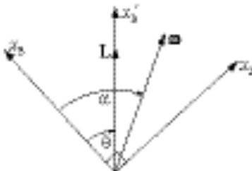
Initially:
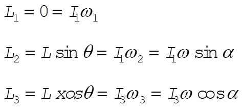
Thus
 (1) (1)
From Eq. (11.102)
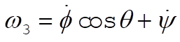
Since 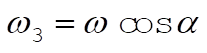 , we have , we have
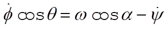 (2) (2)
From Eq. (11.131)
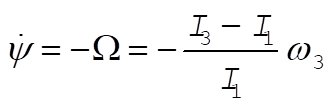
(2) becomes
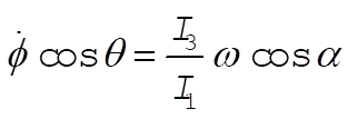 (3) (3)
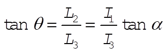
From (1), we may construct the following triangle
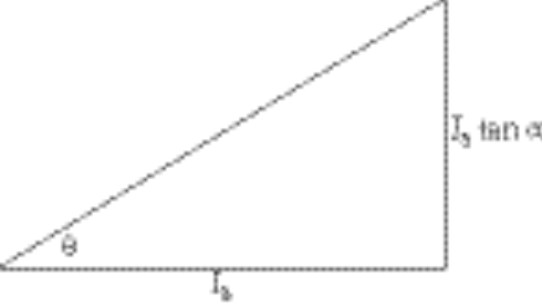
from which 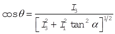
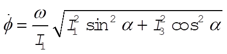
Substituting into (3) gives
�������������������������� 
�������������������������� 11-29. When the motion is vertical q = 0. Then, according to Eqs. (11.153) and (11.154),
 (1) (1)
and using Eq. (11.159), we see that
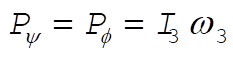 (2) (2)
Also, when q = 0 (and  ), the energy is [see Eq. (11.158)] ), the energy is [see Eq. (11.158)]
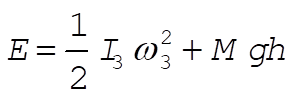 (3) (3)
Furthermore, referring to Eq. (11.160),
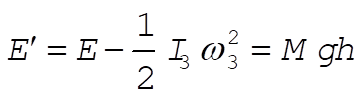 (3) (3)
If we wish to examine the behavior of the system near q = 0 in order to determine the conditions for stability, we can use the values of  , ,  , and E¢ for q = 0 in Eq. (11.161). Thus, , and E¢ for q = 0 in Eq. (11.161). Thus,
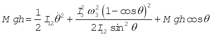 (5) (5)
Changing the variable to z = cos q and rearranging, Eq. (5) becomes
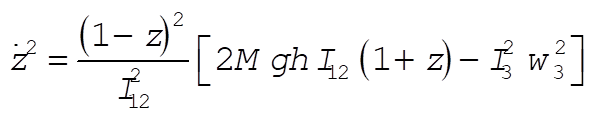 (6) (6)
The questions concerning stability can be answered by examining this expression. First, we note that for physically real motion we must have  . Now, suppose that the top is spinning very rapidly, i.e., that . Now, suppose that the top is spinning very rapidly, i.e., that  is large. Then, the term in the square brackets will be negative. In such a case, the only way to maintain the condition is large. Then, the term in the square brackets will be negative. In such a case, the only way to maintain the condition  is to have z = 1, i.e., q = 0. Thus, the motion at q = 0 will be stable as long as is to have z = 1, i.e., q = 0. Thus, the motion at q = 0 will be stable as long as
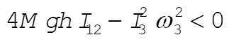 (7) (7)
or,
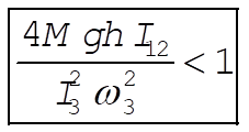 (8) (8)
Suppose now that the top is set spinning with q = 0 but with  sufficiently small that the condition in Eq. (8) is not met. Any small disturbance away from q = 0 will then give sufficiently small that the condition in Eq. (8) is not met. Any small disturbance away from q = 0 will then give  a negative value and q will continue to increase; i.e., the motion is unstable. In fact, q will continue until z reaches a value a negative value and q will continue to increase; i.e., the motion is unstable. In fact, q will continue until z reaches a value  that again makes the square brackets equal to zero. This is a turning point for the motion and nutation between z = 1 and that again makes the square brackets equal to zero. This is a turning point for the motion and nutation between z = 1 and  will result. will result.
From this discussion it is evident that there exists a critical value for the angular velocity,  , such that for , such that for  the motion is stable and for the motion is stable and for  there is nutation: there is nutation:
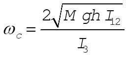 (9) (9)
If the top is set spinning with  and q = 0, the motion will be stable. But as friction slows the top, the critical angular velocity will eventually be reached and nutation will set in. This is the case of the “sleeping top.” and q = 0, the motion will be stable. But as friction slows the top, the critical angular velocity will eventually be reached and nutation will set in. This is the case of the “sleeping top.”
Chapter 12
12-1.
The equations of motion are
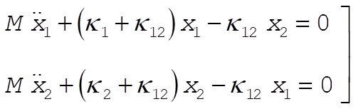 (1) (1)
We attempt a solution of the form
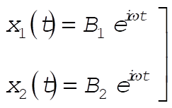 (2) (2)
Substitution of (2) into (1) yields
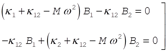 (3) (3)
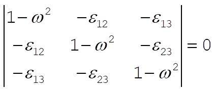
In order for a non-trivial solution to exist, the determinant of coefficients of  and and  must vanish. This yields must vanish. This yields
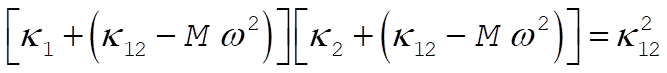 (4) (4)
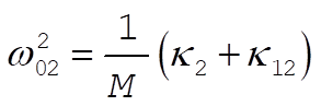
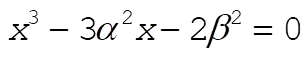
from which we obtain
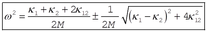 (5) (5)
This result reduces to 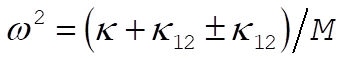 for the case for the case  (compare Eq. (12.7)]. (compare Eq. (12.7)].
If  were held fixed, the frequency of oscillation of were held fixed, the frequency of oscillation of  would be would be
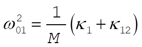 (6) (6)
while in the reverse case,  would oscillate with the frequency would oscillate with the frequency
 (7) (7)
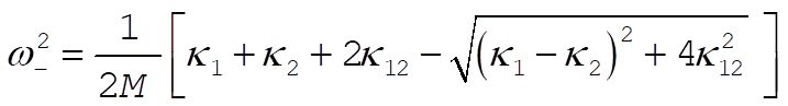
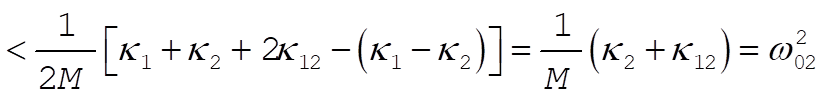
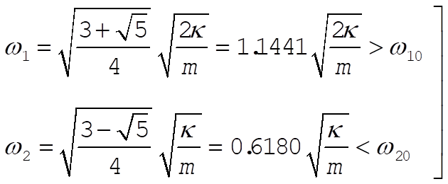
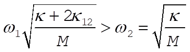
Comparing (6) and (7) with the two frequencies,  and and  , given by (5), we find , given by (5), we find
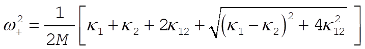
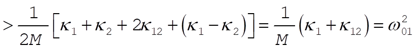 (8) (8)
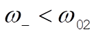
so that
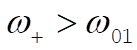 (9) (9)
Similarly,
 (10) (10)
so that
 (11) (11)
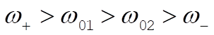
If 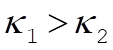 , then the ordering of the frequencies is , then the ordering of the frequencies is
�������������������������� 
12-7.
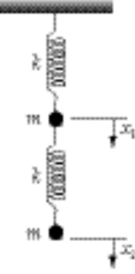
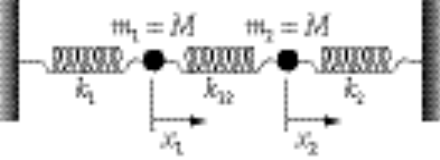
We define the coordinates  and and  as in the diagram. Including the constant downward gravitational force on the masses results only in a displacement of the equilibrium positions and does not affect the eigenfrequencies or the normal modes. Therefore, we write the equations of motion without the gravitational terms: as in the diagram. Including the constant downward gravitational force on the masses results only in a displacement of the equilibrium positions and does not affect the eigenfrequencies or the normal modes. Therefore, we write the equations of motion without the gravitational terms:
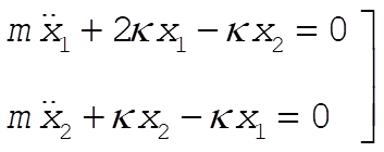 (1) (1)
Assuming a harmonic time dependence for  and and  in the usual way, we obtain in the usual way, we obtain
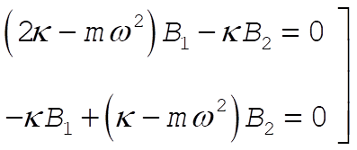 (2) (2)
Solving the secular equation, we find the eigenfrequencies to be
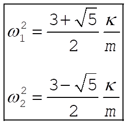 (3) (3)
Substituting these frequencies into (2), we obtain for the eigenvector components
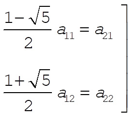 (4) (4)
For the initial conditions 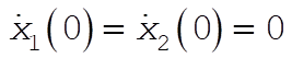 , the normal coordinates are , the normal coordinates are
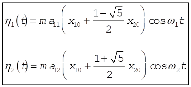 (5) (5)
Therefore, when  , ,  and the system oscillates in Mode 1, the antisymmetrical mode. When and the system oscillates in Mode 1, the antisymmetrical mode. When  , ,  and the system oscillates in Mode 2, the symmetrical mode. and the system oscillates in Mode 2, the symmetrical mode.
When mass 2 is held fixed, the equation of motion of mass 1 is
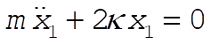 (6) (6)
and the frequency of oscillation is
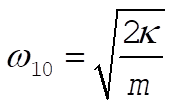 (7) (7)
When mass 1 is held fixed, the equation of motion of mass 2 is
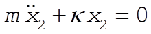 (8) (8)
and the frequency of oscillation is
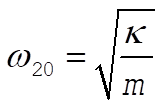 (9) (9)
Comparing these frequencies with  and and  we find we find
Thus, the coupling of the oscillators produces a shift of the frequencies away from the uncoupled frequencies, in agreement with the discussion at the end of Section 12.2.
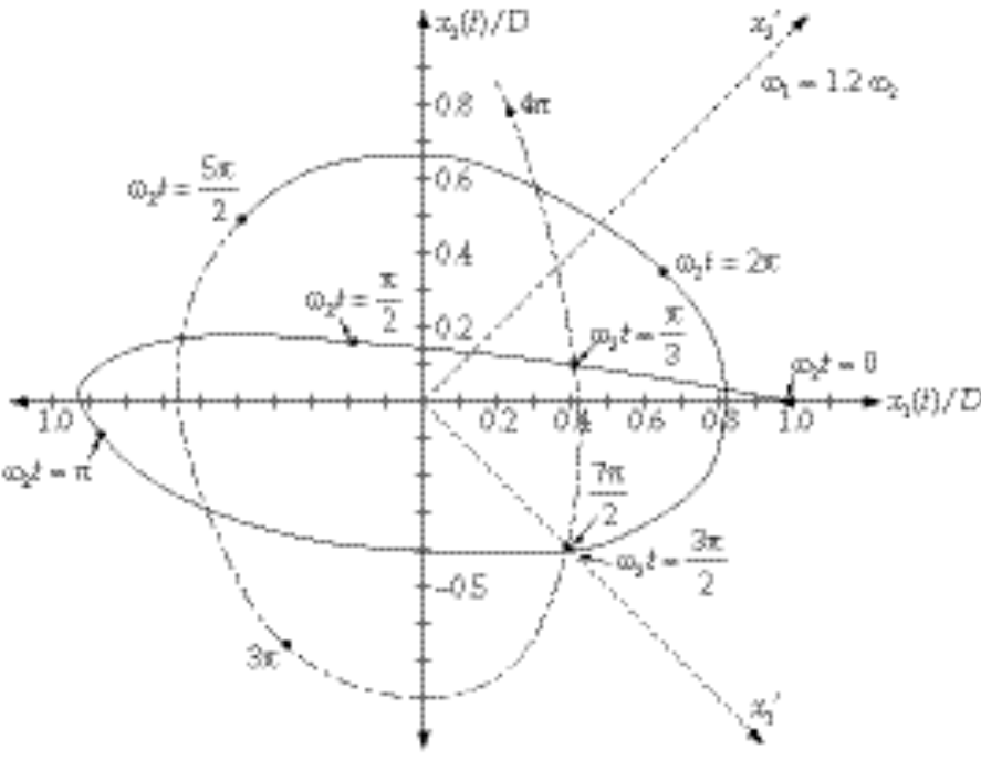
12-9. The general solutions for  and and  are given by Eqs. (12.10). For the initial conditions we choose oscillator 1 to be displaced a distance D from its equilibrium position, while oscillator 2 is held at are given by Eqs. (12.10). For the initial conditions we choose oscillator 1 to be displaced a distance D from its equilibrium position, while oscillator 2 is held at  , and both are released from rest: , and both are released from rest:
 (1) (1)
Substitution of (1) into Eq. (12.10) determines the constants, and we obtain
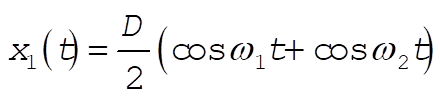 (2) (2)
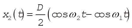 (3) (3)
where
 (4) (4)
As an example, take  ; ;  vs. vs.  is plotted below for this case. is plotted below for this case.
It is possible to find a rotation in configuration space such that the projection of the system point onto each of the new axes is simple harmonic.
By inspection, from (2) and (3), the new coordinates must be
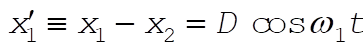 (5) (5)
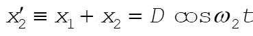 (6) (6)
These new normal axes correspond to the description by the normal modes. They are represented by dashed lines in the graph of the figure.
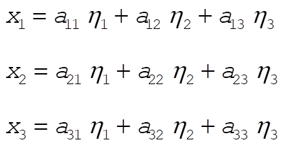
12-17.
Following the procedure outlined in section 12.6:
Thus
Thus we must solve
This reduces to
or
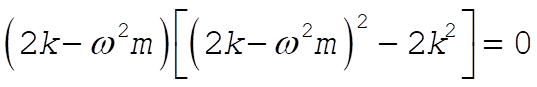
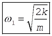
If the first term is zero, then we have
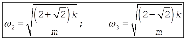
If the second term is zero, then
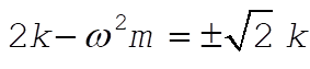
which leads to
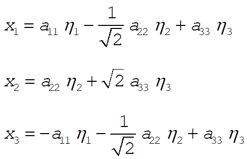
To get the normal modes, we must solve
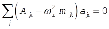
For k = 1 this gives:
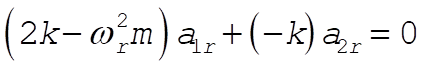
Substituting for each value of r gives
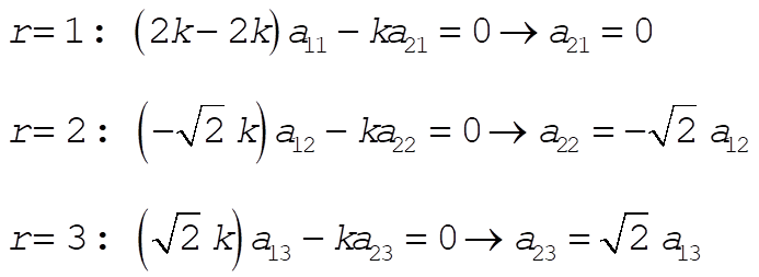
Doing the same for k = 2 and 3 yields
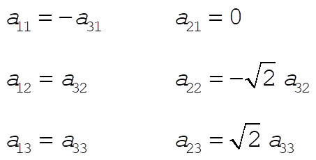
The equations
can thus be written as
We get the normal modes by solving these three equations for  , ,  , ,  : :
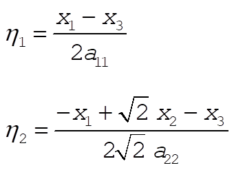
and
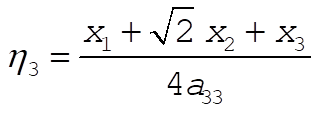
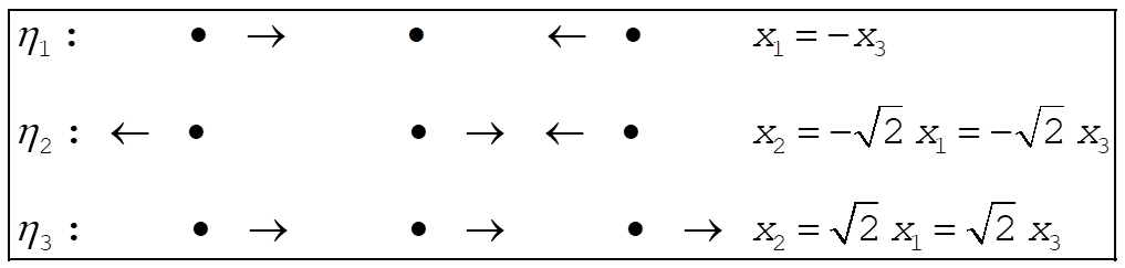
The normal mode motion is as follows
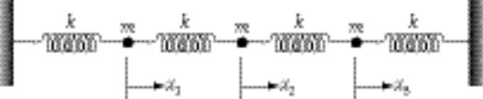
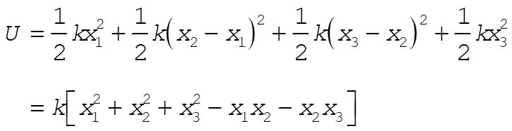
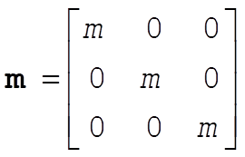
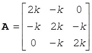
12-19. With the given expression for U, we see that  has the form has the form
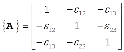 (1) (1)
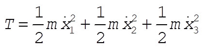
The kinetic energy is
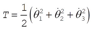 (2) (2)
so that  is is
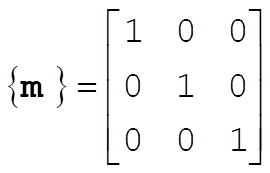 (3) (3)
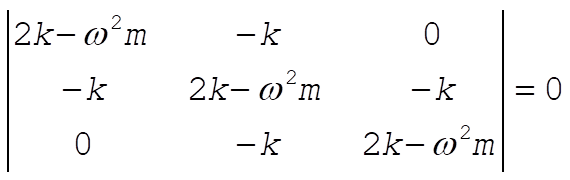
The secular determinant is
 (4) (4)
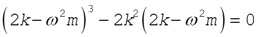
Thus,
 (5) (5)
This equation is of the form (with 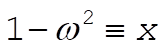 ) )
 (6) (6)
which has a double root if and only if
 (7) (7)
Therefore, (5) will have a double root if and only if
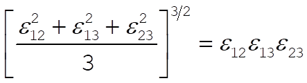 (8) (8)
This equation is satisfied only if
 (9) (9)
Consequently, there will be no degeneracy unless the three coupling coefficients are identical.
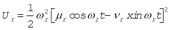
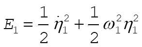
12-23. The total energy of the r-th normal mode is
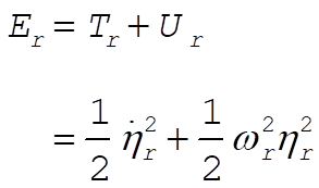 (1) (1)
where
 (2) (2)
Thus,
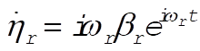 (3) (3)
In order to calculate  and and  , we must take the squares of the real parts of , we must take the squares of the real parts of  and and  : :
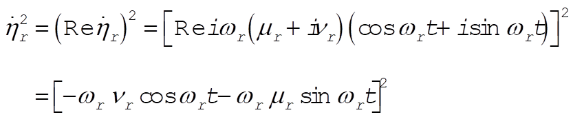 (4) (4)
so that
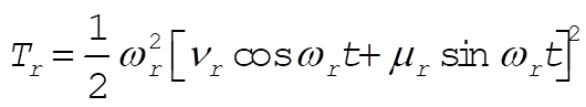 (5) (5)
Also
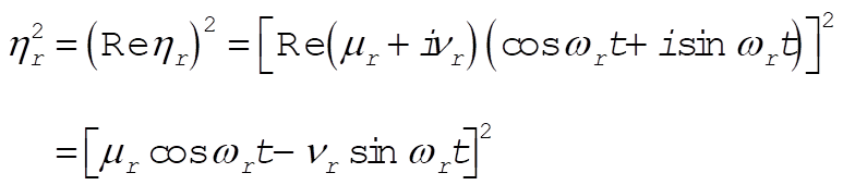 (6) (6)
so that
 (7) (7)
Expanding the squares in  and and  , and then adding, we find , and then adding, we find
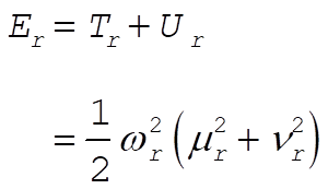
Thus,
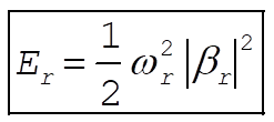 (8) (8)
So that the total energy associated with each normal mode is separately conserved.
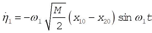
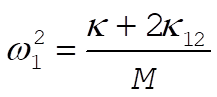
For the case of Example 12.3, we have for Mode 1
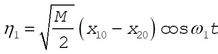 (9) (9)
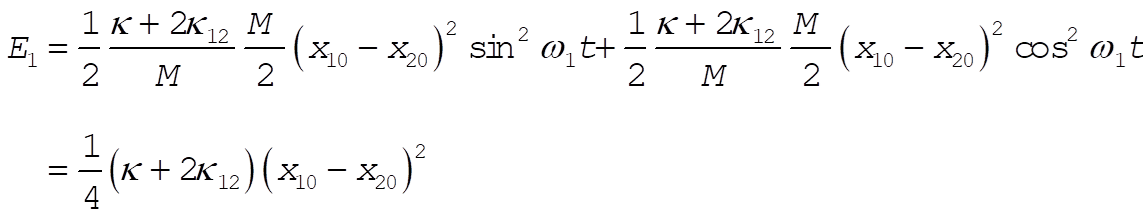
Thus,
 (10) (10)
Therefore,
 (11) (11)
But
 (12) (12)
so that
 (13) (13)
which is recognized as the value of the potential energy at t = 0. [At t = 0,  , so that the total energy is , so that the total energy is  .] .]
At this point, you can go to the 3309 page,
the UH Space Physics Group
Web Site, or my personal Home Page.
Edgar A. Bering, III ,
Edgar A. Bering, III , <eabering@uh.edu>
|
 Homework 13