|
| |
Physics 3309 Homework 6
Chapter 4
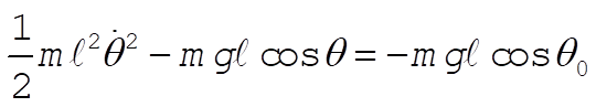
4-7. Let us start with the equation of motion for the simple pendulum:
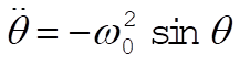 (1) (1)
where 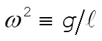 . Put this in terms of the horizontal component by setting . Put this in terms of the horizontal component by setting 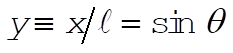 . Solving for q and taking time derivatives, we obtain . Solving for q and taking time derivatives, we obtain
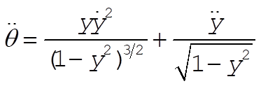 (2) (2)
Since we are keeping terms to third order, we need to get a better handle on the  term. Help comes from the conservation of energy: term. Help comes from the conservation of energy:
 (3) (3)
where  is the maximum angle the pendulum makes, and serves as a convenient parameter that describes the total energy. When written in terms of is the maximum angle the pendulum makes, and serves as a convenient parameter that describes the total energy. When written in terms of  , the above equation becomes (with the obvious definition for , the above equation becomes (with the obvious definition for  ) )
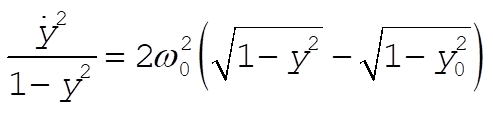 (4) (4)
Substituting (4) into (2), and the result into (1) gives
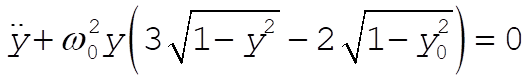 (5) (5)
Using the binomial expansion of the square roots and keeping terms up to third order, we can obtain for the x equation of motion
ĀĀĀĀĀĀĀĀĀĀĀĀĀĀĀĀĀĀĀĀĀĀĀĀĀĀ 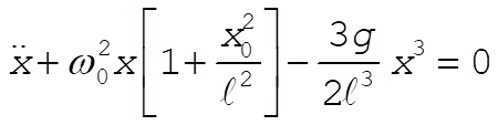
ĀĀĀĀĀĀĀĀĀĀĀĀĀĀĀĀĀĀĀĀĀĀĀĀĀĀ
4-11. The three-cycle does indeed occur where indicated in the problem, and does turn chaotic near the 80th iteration. This value is approximate, however, and depends on the precision at which the calculations are performed. The behavior returns to a three-cycle near the 200th iteration, and stays that way until approximately the 270th iteration, although some may see it continue past the 300th.
ĀĀĀĀĀĀĀĀĀĀĀĀ 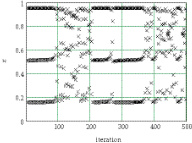
4-13.
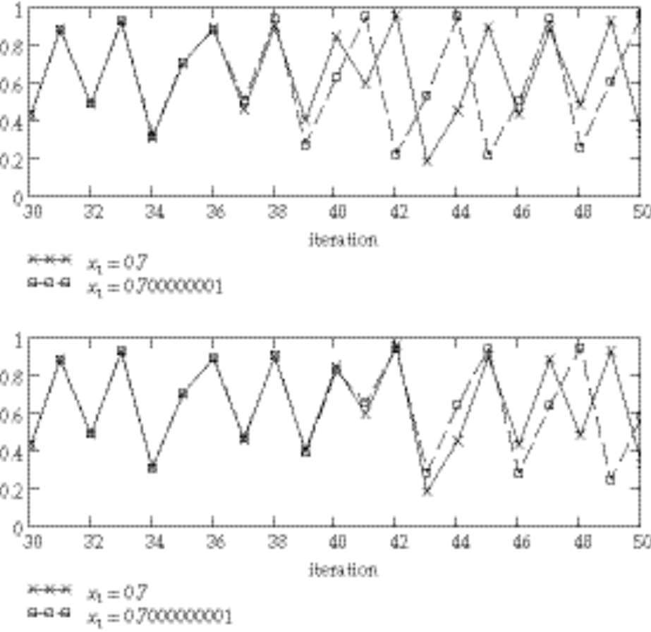
The plots are created by iteration on the initial values of (i) 0.7, (ii) 0.700000001, and (iii) 0.7000000001, using the equation
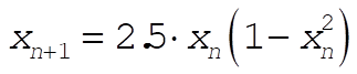 (1) (1)
A subset of the iterates from (i) and (ii) are plotted together, and clearly diverge by n = 39. The plot of (i) and (iii) clearly diverge by n = 43.
4‑19. From the definition in Equation (4.52) the Lyapunov exponent is given by
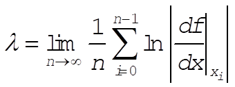 (1) (1)
The tent map is defined as
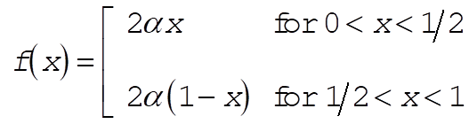 (2) (2)
This gives 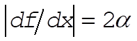 , so we have , so we have
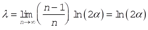 (3) (3)
As indicated in the discussion below Equation (4.52), chaos occurs when l is positive: 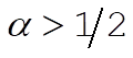 for the tent map. for the tent map.
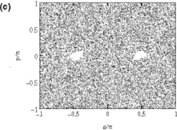
4-23. The Chirikov map is defined by
 (1) (1)
 (2) (2)
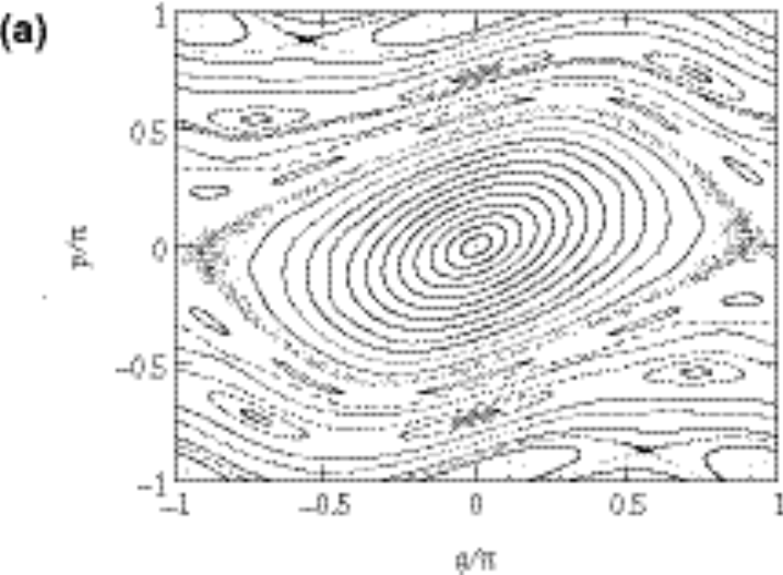
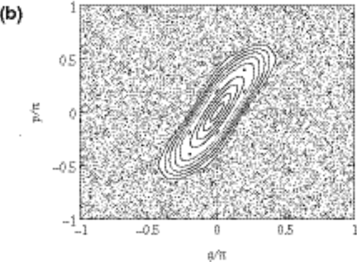
The results one should get from doing this problem should be some subset of the results shown in figures (a), (b), and (c) (for K = 0.8, 3.2, and 6.4, respectively). These were actually generated using some not-so-random initial points so that a reasonably complete picture could be made. What look to be phase paths in the figures are actually just different points that come from iterating on a single initial condition. For example, in figure (a), an ellipse about the origin (just pick one) comes from iterating on any one of the points on it. Above the ellipses is chaotic orbit, then a five ellipse orbit (all five come from a single initial condition), etc. The case for K = 3.2 is similar except that there is an orbit outside of which the system is always undergoing chaotic motion. Finally, for K = 6.4 the entire space is filled with chaotic orbits, with the exception of two small lobes. Inside of these lobes are regular orbits (the ones in the left are separate from the ones in the right).
Chapter 5
5-3. In order to remove a particle from the surface of the Earth and transport it infinitely far away, the initial kinetic energy must equal the work required to move the particle from  to r = ¥ against the attractive gravitational force: to r = ¥ against the attractive gravitational force:
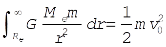 (1) (1)
where  and and  are the mass and the radius of the Earth, respectively, and are the mass and the radius of the Earth, respectively, and  is the initial velocity of the particle at is the initial velocity of the particle at  . .
Solving (1), we have the expression for  : :
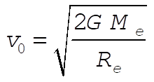 (2) (2)
Substituting  , ,  , ,  , we have , we have
ĀĀĀĀĀĀĀĀĀĀĀĀĀĀĀĀĀĀĀĀĀĀĀĀĀĀ 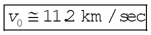
5-7.
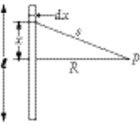
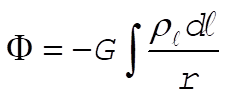
The contribution to the potential at P from a small line element is
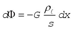 (1) (1)
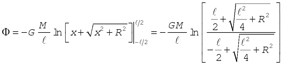
where 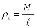 is the linear mass density. Integrating over the whole rod, we find the potential is the linear mass density. Integrating over the whole rod, we find the potential
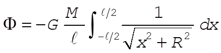 (2) (2)
Using Eq. (E.6), Appendix E, we have
ĀĀĀĀĀĀĀĀĀĀĀĀ ĀĀĀĀĀĀĀĀĀĀĀĀ 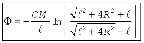
5-9.
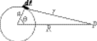
The contribution to the potential at the point P from a small line element dl is
 (1) (1)
where  is the linear mass density which is expressed as is the linear mass density which is expressed as 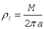 . Using . Using 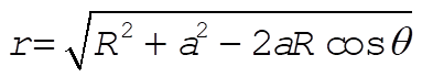 and dl = adq, we can write (1) as and dl = adq, we can write (1) as
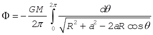 (2) (2)
This is the general expression for the potential.
If R is much greater than a, we can expand the integrand in (2) using the binomial expansion:
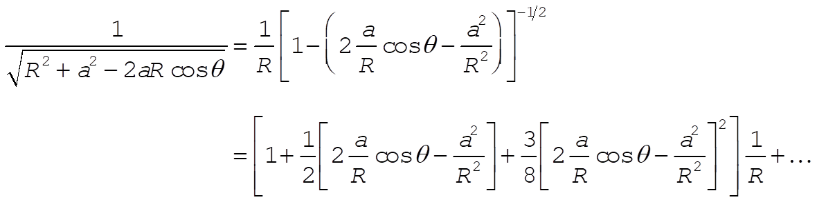 (3) (3)
If we neglect terms of order  and higher in (3), the potential becomes and higher in (3), the potential becomes
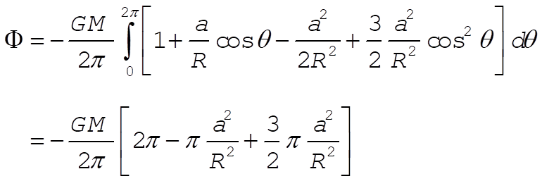 (4) (4)
or,
 (5) (5)
We notice that the first term in (5) is the potential when mass M is concentrated in the center of the ring. Of course this is a very rough approximation and the first correction term is  . .
At this point, you can go to the 3309 page,
the UH Space Physics Group
Web Site, or my personal Home Page.
Edgar A. Bering, III ,
Edgar A. Bering, III , <eabering@uh.edu>
|
 Homework 6