|
| |
Physics 3309 Homework 5
Chapter 3
3-19. The amplitude of a damped oscillator is [Eq. (3.59)]
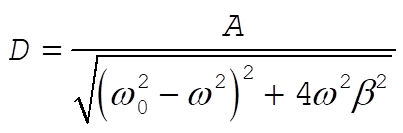 (1) (1)
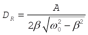
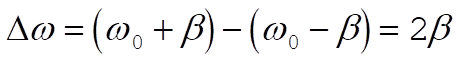
At the resonance frequency, 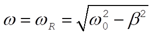 , D becomes , D becomes
 (2) (2)
Let us find the frequency, w = w¢, at which the amplitude is 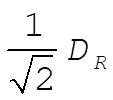 : :
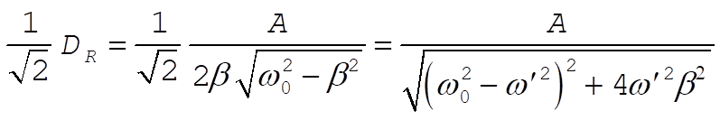 (3) (3)
Solving this equation for w¢, we find
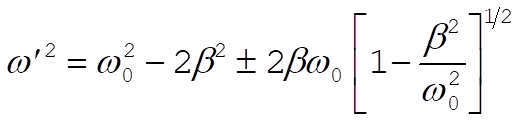 (4) (4)
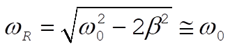
For a lightly damped oscillator, b is small and the terms in  can be neglected. Therefore, can be neglected. Therefore,
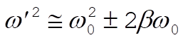 (5) (5)
or,
 (6) (6)
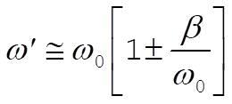
which gives
 (7) (7)
We also can approximate  for a lightly damped oscillator: for a lightly damped oscillator:
 (8) (8)
Therefore, Q for a lightly damped oscillator becomes
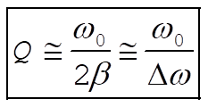 (9) (9)
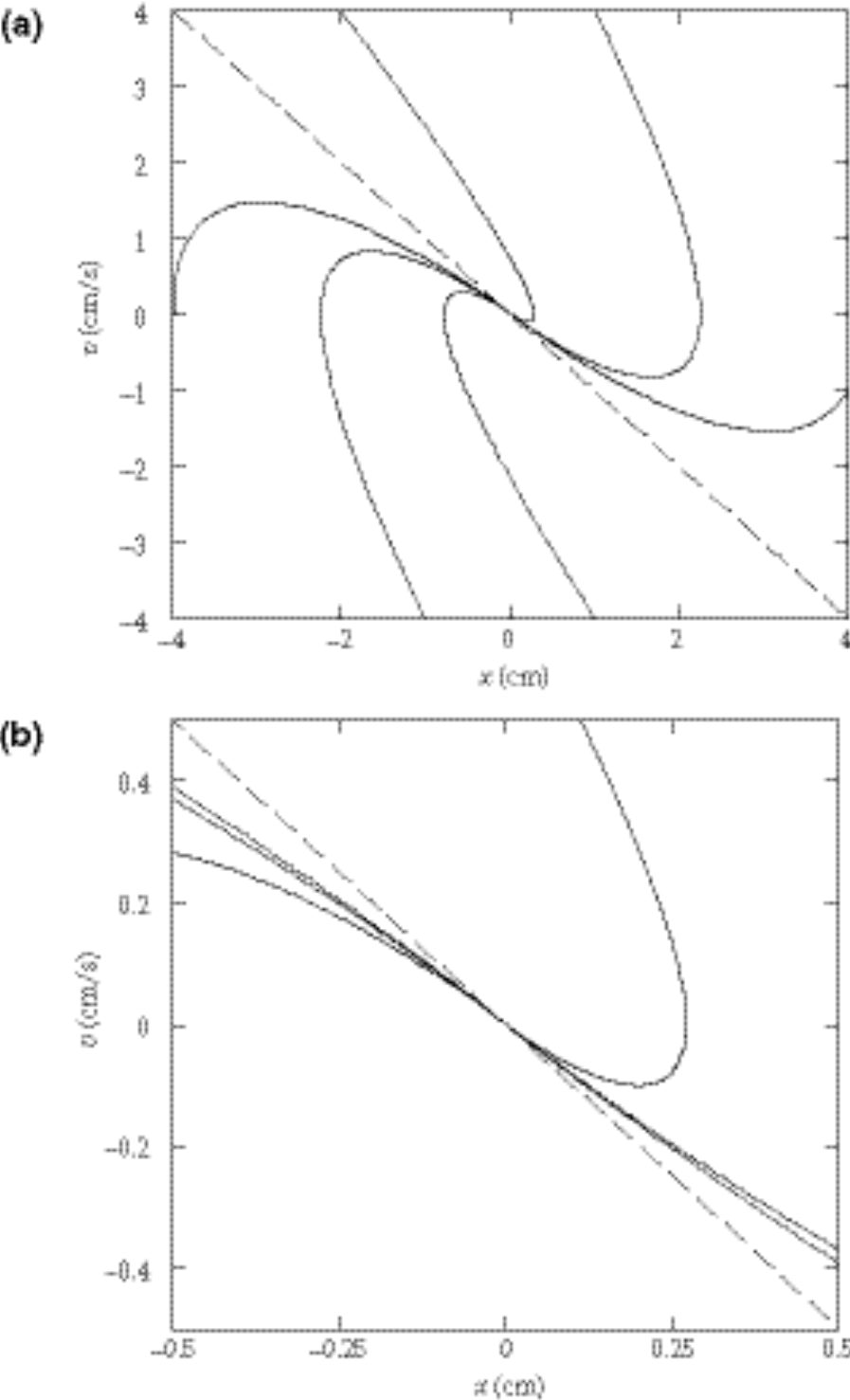
3-21. We want to plot Equation (3.43), and its derivative:
 (1) (1)
 (2) (2)
where A and B can be found in terms of the initial conditions
 (3) (3)
 (4) (4)
The initial conditions used to produce figure (a) were  , ,  , ,  , ,  , ,  , and , and  , where we take all x to be in cm, all v in , where we take all x to be in cm, all v in  , and , and  . Figure (b) is a magnified view of figure (a). The dashed line is the path that all paths go to asymptotically as t ® ¥. This can be found by taking the limits. . Figure (b) is a magnified view of figure (a). The dashed line is the path that all paths go to asymptotically as t ® ¥. This can be found by taking the limits.
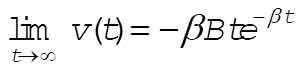 (5) (5)
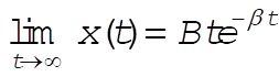 (6) (6)
so that in this limit, v = –bx, as required.
������������ 
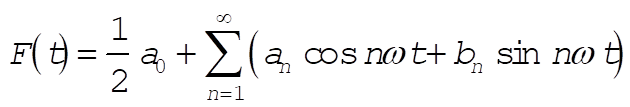
3-27. From Eq. (3.89),
 (1) (1)
We write
 (2) (2)
which can also be written using trigonometric relations as
 (3) (3)
Comparing (3) with (2), we notice that if there exists a set of coefficients  such that such that
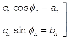 (4) (4)
then (2) is equivalent to (1). In fact, from (4),
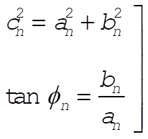 (5) (5)
with  and and  as given by Eqs. (3.91). as given by Eqs. (3.91).
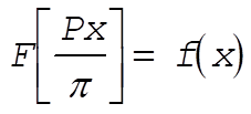
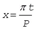
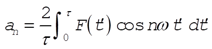
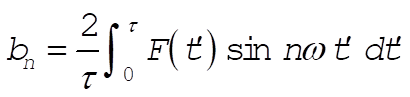
3-29. In order to Fourier analyze a function of arbitrary period, say 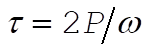 instead of instead of  , proportional change of scale is necessary. Analytically, such a change of scale can be represented by the substitution , proportional change of scale is necessary. Analytically, such a change of scale can be represented by the substitution
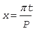 or or 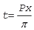 (1) (1)
for when t = 0, then x = 0, and when 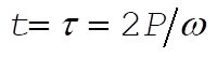 , then , then 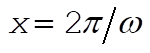 . .
Thus, when the substitution 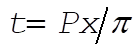 is made in a function F(t) of period is made in a function F(t) of period 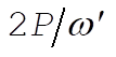 , we obtain the function , we obtain the function
 (2) (2)
and this, as a function of x, has a period of  . Now, f(x) can, of course, be expanded according to the standard formula, Eq. (3.91): . Now, f(x) can, of course, be expanded according to the standard formula, Eq. (3.91):
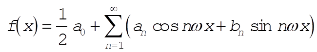 (3) (3)
where
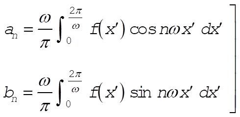 (4) (4)
If, in the above expressions, we make the inverse substitutions
 and and 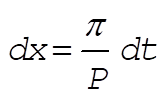 (5) (5)
the expansion becomes
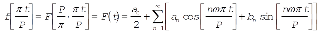 (6) (6)
and the coefficients in (4) become
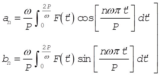 (7) (7)
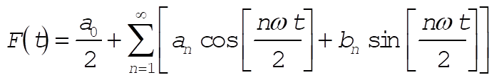
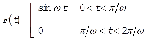
For the case corresponding to this problem, the period of F(t) is  , so that P = 2p. Then, substituting into (7) and replacing the integral limits 0 and t by the limits , so that P = 2p. Then, substituting into (7) and replacing the integral limits 0 and t by the limits  and and  , we obtain , we obtain
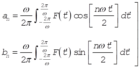 (8) (8)
and substituting into (6), the expansion for F(t) is
 (9) (9)
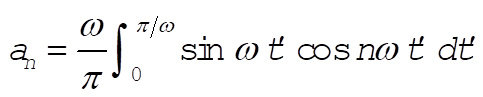
Substituting F(t) into (8) yields
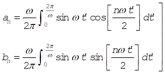 (10) (10)
Evaluation of the integrals gives
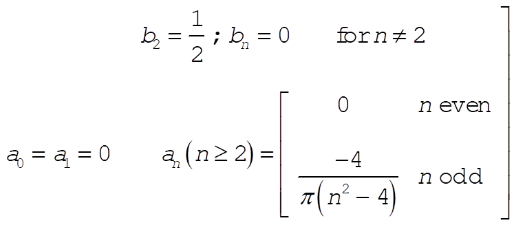 (11) (11)
and the resulting Fourier expansion is
������������  (12) (12)
3-33.
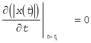
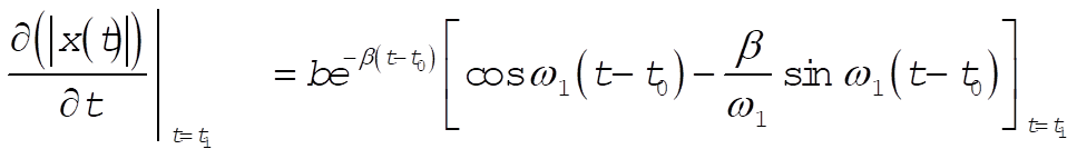
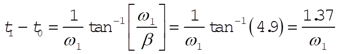
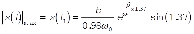
a) In order to find the maximum amplitude of the response function shown in Fig. 3-22, we look for  such that such that  given by Eq. (3.105) is maximum; that is, given by Eq. (3.105) is maximum; that is,
 (1) (1)
From Eq. (3.106) we have
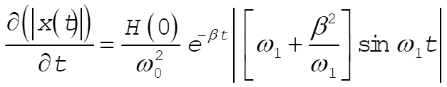 (2) (2)
For  , , 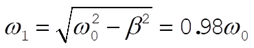 . Evidently, . Evidently, 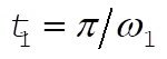 makes (2) vanish. (This is the absolute maximum, as can be seen from Fig. 3-22.) makes (2) vanish. (This is the absolute maximum, as can be seen from Fig. 3-22.)
Then, substituting into Eq. (3.105), the maximum amplitude is given by
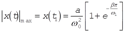 (3) (3)
or,
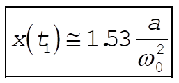 (4) (4)
b) In the same way we find the maximum amplitude of the response function shown in Fig. 3‑24 by using x(t) given in Eq. (3.110); then,
 (5) (5)
If (5) is to vanish,  is given by is given by
 (6) (6)
Substituting (6) into Eq. (3.110), we obtain (for 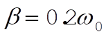 ) )
 (7) (7)
or,
�������������������������� 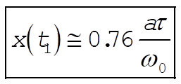 (8) (8)
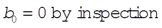
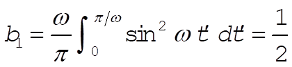
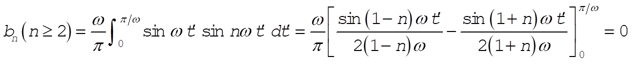
3-39.
From Equations 3.89, 3.90, and 3.91, we have
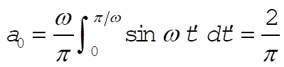
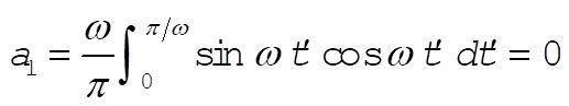
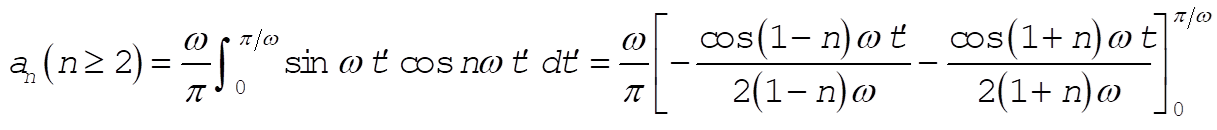
Upon evaluating and simplifying, the result is
 n = 0,1,2,¼ n = 0,1,2,¼
So
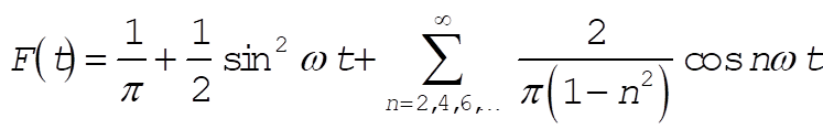
or, letting n ® 2n
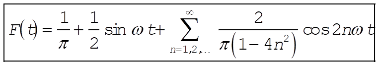
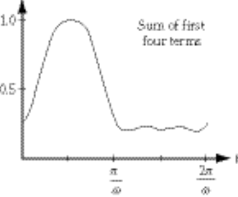
The following plot shows how well the first four terms in the series approximate the function.
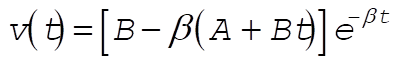
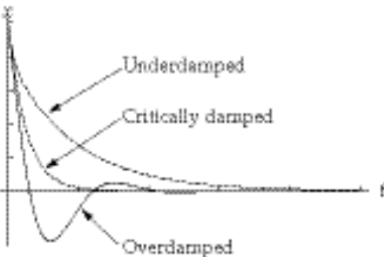
3-41.
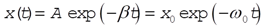
a) The general solution of the given differential equation is (see Equation (3.37))

and
at t = 0,  , , 
 and and 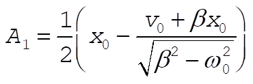 (1) (1)
b)
i) Underdamped, 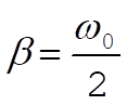
In this case, instead of using above parameterization, it is more convenient to work with the following parameterization
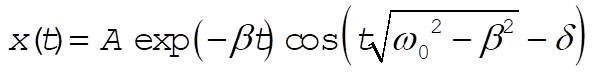 (2) (2)
 (3) (3)
Using initial conditions of x(t) and v(t), we find
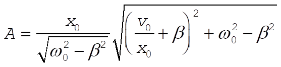 and and 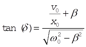
In the case  , and using (6) below we have , and using (6) below we have
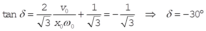
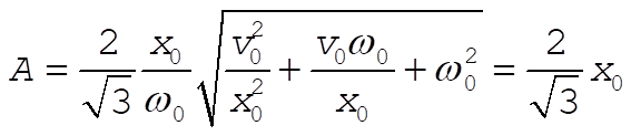
so finally
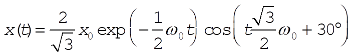 (4) (4)
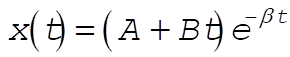
ii) Critically damped,  , using the same parameterization as in i) we have from (2) and (3): , using the same parameterization as in i) we have from (2) and (3):
 (5) (5)
and  (6) (6)
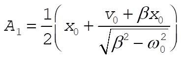
iii) Overdamped,  , returning to the original parameterization (1) we have (always using relation (6)), , returning to the original parameterization (1) we have (always using relation (6)),
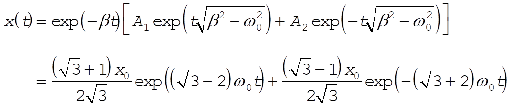 (7) (7)
Below we show sketches for equations (4), (5), (7)
Chapter 4
4-3. The potential 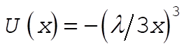 has the form shown in (a) below. The corresponding phase diagram is given in (b): has the form shown in (a) below. The corresponding phase diagram is given in (b):
At this point, you can go to the 3309 page,
the UH Space Physics Group
Web Site, or my personal Home Page.
Edgar A. Bering, III ,
Edgar A. Bering, III , <eabering@uh.edu>
|
 Homework 5